Using extreme ValueTheory and Copulas
to Evaluate Market Risk
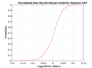
This example shows how to model the market risk of a hypothetical global equity index portfolio with a Monte Carlo simulation technique using a Student's t copula and Extreme Value Theory (EVT). The process first extracts the filtered residuals from each return series with an asymmetric GARCH model, then constructs the sample marginal cumulative distribution function (CDF) of each asset using a Gaussian kernel estimate for the interior and a generalized Pareto distribution (GPD) estimate for the upper and lower tails. A Student's t copula is then fit to the data and used to induce correlation between the simulated residuals of each asset. Finally, the simulation assesses the Value-at-Risk (VaR) of the hypothetical global equity portfolio over a one month horizon.
The raw data consists of 2665 observations of daily closing values of the following representative equity indices spanning the trading dates 27-April-1993 to 14-July-2003:
Canada: TSX Composite (Ticker ^GSPTSE)
France: CAC 40 (Ticker ^FCHI)
Germany: DAX (Ticker ^GDAXI)
Japan: Nikkei 225 (Ticker ^N225)
UK: FTSE 100 (Ticker ^FTSE)
US: S&P 500 (Ticker ^GSPC)
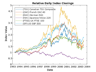
The following plot illustrates the relative price movements of each index. The initial level of each index has been normalized to unity to facilitate the comparison of relative performance, and no dividend adjustments are explicitly taken into account.
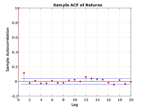
In preparation for subsequent modeling, convert the closing level of each index to daily logarithmic returns (sometimes called geometric, or continuously compounded, returns). Modeling the tails of a distribution with a GPD requires the observations to be approximately independent and identically distributed (i.i.d.). However, most financial return series exhibit some degree of autocorrelation and, more importantly, heteroskedasticity. For example, the sample autocorrelation function (ACF) of the returns associated with the selected index reveal some mild serial correlation
However, the sample ACF of the squared returns illustrates the degree of persistence in variance, and implies that GARCH modeling may significantly condition the data used in the subsequent tail estimation process.
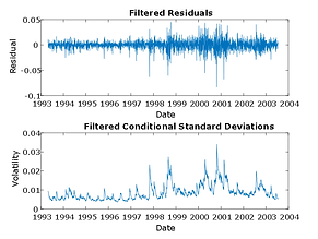
To produce a series of i.i.d. observations, fit a first order autoregressive model to the conditional mean of the returns of each equity index and an asymmetric GARCH model to the conditional variance. The first order autoregressive model compensates for autocorrelation, while the GARCH model compensates for heteroskedasticity.
Having filtered the model residuals from each return series, standardize the residuals by the corresponding conditional standard deviation. These standardized residuals represent the underlying zero-mean, unit-variance, i.i.d. series upon which the EVT estimation of the sample CDF tails is based.
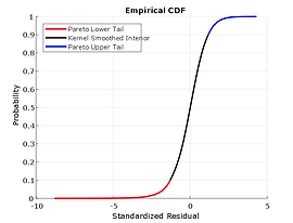
Given the standardized, i.i.d. residuals from the previous step, estimate the empirical CDF of each index with a Gaussian kernel. This smoothes the CDF estimates, eliminating the staircase pattern of unsmoothed sample CDFs. Although non-parametric kernel CDF estimates are well suited for the interior of the distribution where most of the data is found, they tend to perform poorly when applied to the upper and lower tails. To better estimate the tails of the distribution, apply EVT to those residuals that fall in each tail.
Specifically, find upper and lower thresholds such that 10% of the residuals is reserved for each tail. Then fit the amount by which those extreme residuals in each tail fall beyond the associated threshold to a parametric GPD by maximum likelihood. This approach is often referred to as the distribution of exceedances or peaks over threshold method.
Given the exceedances in each tail, optimize the negative log-likelihood function to estimate the tail index (zeta) and scale (beta) parameters of the GPD.
Given the standardized residuals, now estimate the scalar degrees of freedom parameter (DoF) and the linear correlation matrix (R) of the t copula. Given the parameters of a t copula, now simulate jointly dependent equity index returns by first simulating the corresponding dependent standardized residuals.
Then, by extrapolating into the GP tails and interpolating into the smoothed interior, transform the uniform variates to standardized residuals via the inversion of the semi-parametric marginal CDF of each index. This produces simulated standardized residuals consistent with those obtained from the AR(1) + GJR(1,1) filtering process above. These residuals are independent in time but dependent at any point in time. Each column of the simulated standardized residuals array represents an i.i.d. univariate stochastic process when viewed in isolation, whereas each row shares the rank correlation induced by the copula.
Finally, given the simulated returns of each index, form an equally weighted global index portfolio composed of the individual indices (a global index of country indices). Since we are working with daily logarithmic returns, the cumulative returns over the risk horizon are simply the sums of the returns over each intervening period. Also note that the portfolio weights are held fixed throughout the risk horizon, and that the simulation ignores any transaction costs required to rebalance the portfolio (the daily rebalancing process is assumed to be self-financing).
